Understanding Real Stable Diffusion Workflows: How It Works Under the Hood
Deep technical explanation of how Stable Diffusion actually works. Learn the denoising process, latent space, VAE, CLIP, U-Net architecture, and...
For my first three months using Stable Diffusion, I had absolutely no idea what I was doing. CFG scale? No clue, just used 7 because everyone else did. Sampling steps? Set it to 30 and hoped for the best. VAE? Honestly thought it was some kind of file format.
I was basically copying workflows from Reddit and Discord, changing prompts, and praying. When something broke, I had zero idea how to fix it. When results looked weird, I just regenerated with a different seed and hoped it would magically work.
Then I spent a weekend actually learning how this stuff works under the hood. The CLIP encoder, the U-Net denoising process, latent space compression, all of it. And suddenly everything clicked. I went from blindly copying workflows to actually understanding why parameters do what they do, which meant I could finally troubleshoot issues and design my own workflows instead of being dependent on others.
- Stable Diffusion works by learning to remove noise in compressed latent space rather than pixel space, reducing computational requirements by 80%
- The architecture combines three neural networks: CLIP (text understanding), U-Net (denoising), and VAE (compression/decompression)
- Each generation step iteratively removes predicted noise, guided by your text prompt encoded as conditioning vectors
- Understanding this architecture explains why certain parameters like CFG scale, sampling steps, and schedulers produce different results
- Platforms like Apatero.com handle all this complexity automatically while giving you full creative control
Quick Answer: Stable Diffusion generates images by starting with random noise and iteratively removing it over 20-50 steps, guided by your text prompt. It works in compressed "latent space" rather than pixel space for efficiency. Three neural networks collaborate: CLIP encodes your text prompt into numerical embeddings, U-Net predicts what noise to remove at each step, and VAE compresses/decompresses between pixel and latent space. This architecture achieves photorealistic results while running on consumer hardware.
What Makes Stable Diffusion Different From Other AI Image Generators?
Stable Diffusion belongs to a category called latent diffusion models, which represents a fundamental breakthrough in how we approach AI image generation. Earlier systems like DALL-E 1 and Imagen worked directly in pixel space, requiring massive computational resources and making them inaccessible to most users.
The Latent Space Innovation: Instead of working with full-resolution images (which might contain millions of pixels), Stable Diffusion compresses images into a much smaller "latent space" representation. Think of it like converting a high-resolution photograph into a compressed format, but instead of JPEG, you're using a learned compression that preserves the information needed for image generation.
This compression happens through a component called the Variational Autoencoder or VAE. The VAE takes a 512x512 pixel image (262,144 values) and compresses it down to a 64x64 latent representation (4,096 values). That's a 64x reduction in data that needs processing, which directly translates to faster generation and lower hardware requirements.
Why This Matters for Users: The decision to work in latent space isn't just an academic curiosity. It's the reason Stable Diffusion can run on a consumer GPU with 8GB of VRAM instead of requiring $100,000 worth of cloud computing. It's why you can generate images in 30 seconds instead of 30 minutes.
When you're working in ComfyUI and you see nodes labeled "VAE Encode" and "VAE Decode," you're witnessing this compression and decompression process. Understanding this helps explain why VAE selection affects image quality, why certain artifacts appear, and why resolution changes impact generation speed the way they do. For practical applications of these concepts in workflow design, check out our beginner's guide to ComfyUI workflows.
While Apatero.com handles all these technical details automatically with optimized defaults, knowing the architecture helps you troubleshoot issues and make informed choices when you need more control.
How Do the Three Core Components Work Together?
Stable Diffusion's architecture relies on three neural networks that each handle a specific part of the generation process. Understanding how they communicate reveals why the system works so well and where limitations come from.
CLIP: The Text Understanding System
CLIP (Contrastive Language-Image Pre-training) is responsible for converting your text prompt into something the neural network can understand. When you type "a golden retriever puppy playing in autumn leaves," CLIP doesn't see English words. It sees a sequence of tokens that need to be converted into numerical vectors.
The CLIP text encoder was trained on millions of image-text pairs, learning associations between visual concepts and their textual descriptions. It produces a 768-dimensional vector (for Stable Diffusion 1.5) or 1024-dimensional vector (for SDXL) that represents the semantic meaning of your prompt.
Why CLIP Matters: This is why prompt engineering works. CLIP learned certain associations during training - "photorealistic," "highly detailed," "trending on ArtStation" - that nudge generation in specific directions. It's also why CLIP understands concepts but struggles with exact counting or spatial relationships. The model learned "several cats" as a concept but not precise numerical quantities.
U-Net: The Denoising Workhorse
The U-Net is the heart of the diffusion process. At each generation step, it looks at the current noisy latent image and your text conditioning, then predicts what noise should be removed to move closer to your desired result.
The architecture is called U-Net because of its shape - it compresses information down through several layers (the downsampling path), then expands it back up (the upsampling path) with skip connections that preserve detail. This design allows it to work at multiple scales simultaneously, handling both overall composition and fine details.
The U-Net receives three inputs at each step:
| Input | Purpose | Typical Size | Impact on Output |
|---|---|---|---|
| Noisy latent image | Current state of generation | 64x64x4 | Visual content being denoised |
| Timestep | How far through denoising process | Single value | Determines denoising strength |
| Text conditioning | Your prompt as CLIP embeddings | 77x768 or 77x1024 | Guides what to denoise toward |
VAE: The Compression/Decompression System
The Variational Autoencoder handles translation between pixel space (what you see) and latent space (where generation happens). It consists of two parts:
The encoder compresses images into latent representations. This happens when you use image-to-image generation or when loading a reference image. The encoder learns to preserve important semantic information while discarding redundant pixel-level details.
The decoder decompresses latent representations back into pixel images. This is the final step of every generation, converting the denoised latent image into the actual picture you see. The decoder's quality directly affects your final image quality, which is why VAE selection matters.
The Communication Flow:
Here's what happens during a typical generation, following the data through each component:
- Your text prompt enters CLIP, which produces conditioning vectors
- Random noise is generated in latent space (64x64x4 for SD 1.5)
- U-Net receives the noise, conditioning, and current timestep
- U-Net predicts what portion of the current image is noise
- Predicted noise is removed from the current latent image
- Steps 3-5 repeat 20-50 times, progressively removing noise
- The final denoised latent passes through VAE decoder
- You receive your finished pixel image
This architecture is why platforms like Apatero.com can optimize so effectively - by understanding the bottlenecks in each component, they can allocate computational resources precisely where needed. For those interested in advanced model customization, our guide on LoRA training in ComfyUI shows how to fine-tune components of this pipeline.
What Actually Happens During the Denoising Process?
The denoising process is where the magic happens, but "magic" obscures some fascinating mathematics and clever engineering. Let's break down what occurs during those 20-50 generation steps.
The Forward Diffusion Process (Training Only):
Before we can denoise, we need to understand how the model was trained. During training, Stable Diffusion learned the reverse of what it does during generation. The researchers took real images and progressively added noise to them over many steps, creating a "noise schedule" that goes from clean image to pure random noise.
The model learned to recognize patterns at different noise levels. Early in the noise schedule (low noise), it learned fine details like texture and small features. Late in the noise schedule (high noise), it learned overall composition and large-scale structure.
The Reverse Process (What You Use):
When you generate an image, you're running this process in reverse. You start with pure noise and progressively remove it, guided by the patterns the model learned during training.
Timestep Breakdown:
| Generation Phase | Timestep Range | What's Being Formed | CFG Impact | Typical Issues |
|---|---|---|---|---|
| Early steps (1-15%) | 999-850 | Overall composition, major objects | High sensitivity | Composition shifts |
| Middle steps (15-70%) | 850-300 | Shapes solidify, colors emerge | Medium sensitivity | Style inconsistencies |
| Late steps (70-95%) | 300-50 | Fine details, textures | Low sensitivity | Oversmoothing |
| Final steps (95-100%) | 50-0 | Minor refinements | Minimal impact | Unnecessary iterations |
Why This Matters for Sampling Steps:
Each step refines the image by removing predicted noise. More steps generally mean more refinement, but there are diminishing returns. The difference between 20 and 30 steps is often dramatic. The difference between 50 and 100 steps is usually imperceptible because the image has already converged to a stable state.
The Role of Schedulers:
The scheduler determines how noise removal is distributed across steps. Different schedulers can produce significantly different results even with the same prompt and seed.
Euler makes linear predictions about noise removal - simple and fast but can miss subtle details.
DPM++ 2M Karras uses more sophisticated mathematics to predict optimal noise removal at each step, often producing better results in fewer steps.
DDIM (Denoising Diffusion Implicit Models) allows deterministic generation - the same seed and prompt always produce identical results, useful for reproducibility.
The choice of scheduler interacts with your number of steps. Some schedulers like DPM++ are optimized for 20-30 steps, while others like Euler might need 40-50 for comparable quality.
Understanding CFG Scale (Classifier-Free Guidance):
CFG scale controls how strongly your text prompt influences generation. Understanding what it actually does requires knowing that the U-Net makes two predictions at each step:
- Conditional prediction: What noise to remove based on your prompt
- Unconditional prediction: What noise to remove with no prompt guidance
CFG scale determines how much to weight the difference between these predictions. A CFG scale of 7 means the model leans heavily toward your prompt but still allows some creative freedom. A CFG scale of 15 means it follows your prompt extremely literally, often at the cost of image quality and natural variation.
| CFG Scale | Effect on Generation | Best Use Cases | Common Problems |
|---|---|---|---|
| 1-3 | Ignores prompt significantly | Creative exploration | Prompt ignored |
| 4-7 | Balanced interpretation | Most general use | None typically |
| 8-12 | Strong prompt adherence | Specific compositions | Oversaturation |
| 13-20 | Extremely literal | Technical requirements | Artifacts, burnout |
This denoising architecture explains why changing parameters mid-generation (through techniques like prompt scheduling or CFG scheduling) can produce interesting effects. You're literally changing the guidance signal while the image is being formed. Advanced workflows on Apatero.com use these techniques automatically to optimize image quality without requiring you to understand the underlying mathematics.
For practical applications of these concepts in video generation, see our comprehensive WAN 2.2 guide which applies similar diffusion principles to temporal data.
Why Does Latent Space Compression Matter So Much?
Latent space is one of those concepts that sounds abstract and theoretical until you realize it's the reason AI image generation became accessible to regular users.
I remember the exact moment this clicked for me. I was trying to generate at 1024x1024 and kept getting these weird repeated patterns, like the AI was tiling wallpaper. Tried everything... different prompts, different seeds, different samplers. Nothing worked. Then I read that the model was trained on 512x512, and working in latent space means it expects a certain size latent representation.
Free ComfyUI Workflows
Find free, open-source ComfyUI workflows for techniques in this article. Open source is strong.
Generated at 512x512 and upscaled instead. Perfect. No more repeated patterns. That's when I actually understood that latent space isn't just some abstract concept... it's the actual mathematical space where all the generation happens, and it has specific expectations.
The Computational Mathematics:
Working in pixel space means every operation happens on the full image resolution. For a 512x512 RGB image, that's 512 x 512 x 3 = 786,432 values to process through the neural network at each denoising step. With 30 steps, you're processing over 23 million values.
Latent space compression reduces that 512x512 image to 64x64x4 = 16,384 values. Same 30 steps means processing only 491,520 values - a 98% reduction in computation.
What Information Gets Preserved:
The VAE encoder doesn't compress randomly. It learned during training to preserve semantically important information while discarding perceptually redundant details. Two images that look different at the pixel level but represent the same visual concept (like two photos of the same dog from slightly different angles) produce similar latent representations.
This semantic compression is why Stable Diffusion can generalize so well. The latent space naturally groups similar concepts together, making it easier for the U-Net to learn relationships between visual ideas and text descriptions.
Latent Space Dimensions:
The standard Stable Diffusion latent space has four channels, compared to three (RGB) for pixel images. These four channels don't map directly to human-interpretable concepts, but research suggests they encode different types of visual information - roughly corresponding to structure, color, texture, and detail, though the actual learned representations are more complex.
Why This Explains Common Behaviors:
Several mysterious behaviors of Stable Diffusion make perfect sense once you understand latent space compression:
Resolution limitations: The VAE was trained on specific resolutions. When you try to generate at very different resolutions (like 2048x2048 from a model trained on 512x512), the latent space no longer matches what the model expects, causing repeated patterns or warped compositions.
VAE selection impact: Different VAEs compress information differently. The MSE VAE prioritizes mathematical accuracy, the EMA VAE produces smoother results, and the kl-f8 VAE (standard for SD 1.5) balances both. Your choice affects what details survive compression and how the final image looks.
Latent interpolation: Because latent space represents images as compact vectors, you can blend between images by mathematically averaging their latent representations. This is how prompt blending, style mixing, and certain animation techniques work in practice. Our guide on AnimateDiff with IPAdapter uses these latent space techniques for character-consistent animations.
Speed differences: Image-to-image generation starts from an encoded latent representation rather than pure noise, reducing the denoising range. This is why image-to-image at 70% denoising strength is much faster than text-to-image - you're only doing 15 denoising steps instead of 30.
Practical Implications:
Understanding latent space helps you debug quality issues:
| Problem | Latent Space Cause | Solution |
|---|---|---|
| Blurry details | VAE decoder limitations | Use better VAE or higher resolution |
| Repeated patterns | Resolution mismatch with latent expectations | Generate at trained resolutions |
| Color shifts | VAE color space encoding | Switch VAE or adjust in post-processing |
| Artifacts in upscaling | Latent space interpolation issues | Use proper upscaling models |
When you're working in ComfyUI and you see a "Latent Preview" node showing a blurry version of your generation in progress, you're literally seeing the latent space representation decoded in real-time. It looks blurry because the VAE decoder hasn't refined it yet - the actual information is there in the latent representation.
While Apatero.com selects optimal VAE settings automatically based on your generation parameters, understanding these relationships helps you troubleshoot issues and make informed decisions when you need precise control.
How Do Different Sampling Methods Change Your Results?
Sampling methods determine the mathematical approach used to remove noise at each step. The choice isn't just academic - different samplers can produce noticeably different images from the same prompt and seed.
Deterministic vs. Stochastic Samplers:
Want to skip the complexity? Apatero gives you professional AI results instantly with no technical setup required.
Some samplers are deterministic, meaning the same seed and prompt produce identical results every time. Others are stochastic, introducing controlled randomness that can vary results slightly even with identical settings.
Deterministic samplers:
- DDIM (Denoising Diffusion Implicit Models)
- PLMS (Pseudo Linear Multistep)
- UniPC
Stochastic samplers:
- Euler
- Euler Ancestral
- DPM++ variants
- Heun
Deterministic samplers are crucial for reproducibility. If you're trying to perfect a specific image by adjusting prompts, deterministic samplers ensure changes come from your modifications, not random variation.
Stochastic samplers often produce more natural-looking results by introducing slight variations that prevent overly smooth or repetitive patterns. The "ancestral" variants (Euler a, DPM++ 2S a) add controlled noise at each step, increasing variation.
Sampler Comparison:
| Sampler | Speed | Quality | Best For | Step Count | Behavior |
|---|---|---|---|---|---|
| Euler | Fast | Good | Quick tests | 20-40 | Simple, predictable |
| Euler Ancestral | Fast | Very Good | General use | 20-40 | Natural variation |
| DPM++ 2M Karras | Medium | Excellent | High quality | 20-30 | Efficient convergence |
| DPM++ SDE Karras | Slow | Excellent | Fine detail | 25-40 | Maximum detail |
| DDIM | Fast | Good | Reproducibility | 30-50 | Deterministic |
| UniPC | Very Fast | Good | Speed priority | 15-25 | Efficient but newer |
How Samplers Actually Work:
Euler is the simplest approach, using first-order approximations to predict the next denoising step. Think of it like predicting where a ball will land by looking at its current velocity - accurate for small steps but can accumulate errors over many iterations.
Heun improves on Euler by making a prediction, testing it, then averaging the results - like measuring twice and cutting once. This requires two neural network evaluations per step, making it slower but more accurate.
DPM++ (Diffusion Probabilistic Models Plus Plus) uses second-order approximations, considering both current velocity and acceleration. This allows it to make better predictions about optimal noise removal, often reaching high-quality results in fewer steps.
The Karras suffix refers to a specific noise schedule developed by researcher Tero Karras. Karras noise schedules typically produce better results by changing how noise is distributed across timesteps, with more refinement happening in the middle steps where it has the greatest impact.
SDE (Stochastic Differential Equation) variants introduce controlled randomness based on mathematical modeling of diffusion as a continuous process. This often produces more natural textures and avoids the overly smooth results that can come from purely deterministic approaches.
Practical Selection Guide:
For testing and iteration, use Euler or Euler Ancestral with 20-25 steps. They're fast enough for rapid experimentation while producing acceptable quality.
For final high-quality renders, use DPM++ 2M Karras with 25-30 steps. This hits the sweet spot of quality and efficiency for most use cases.
For maximum detail and realism, use DPM++ SDE Karras with 30-40 steps, accepting the slower generation time for superior results.
For reproducible results (like when doing batch processing or A/B testing), use DDIM with 40-50 steps, ensuring identical seeds produce identical outputs.
Why This Matters for Workflows:
Understanding sampler behavior helps explain why your workflow produces different results when you change samplers. It's not that one is "wrong" - they're solving the denoising problem using different mathematical approaches, each with tradeoffs.
When you're using advanced workflows with techniques like regional prompting or mask-based composition, sampler choice becomes even more important because you're asking the model to handle complex conditional generation. Stochastic samplers often handle these scenarios better by avoiding getting stuck in local minima.
Earn Up To $1,250+/Month Creating Content
Join our exclusive creator affiliate program. Get paid per viral video based on performance. Create content in your style with full creative freedom.
Platforms like Apatero.com select samplers automatically based on your generation type and quality settings, but understanding the differences helps you make informed choices when you need manual control.
What Are the Practical Implications of Understanding This Architecture?
Knowing how Stable Diffusion works under the hood isn't just academic knowledge - it directly translates to better results and more efficient workflows. Let's connect the technical details to practical improvements you can make today.
Better Parameter Selection:
Last week a client said my generations looked "oversaturated and artificial." Old me would've just... tried different prompts? Changed the seed 50 times? But now I knew exactly what was happening. I was running CFG scale at 15 because I wanted "strong prompt adherence." But high CFG amplifies the difference between conditional and unconditional predictions, which causes exactly that oversaturated, artificial look.
Dropped CFG to 8, same prompt, same seed, problem solved. Five minutes instead of hours of frustrated regeneration.
When you understand that CFG scale controls the balance between conditional and unconditional predictions, you stop treating it like a mysterious "prompt strength" slider and start using it strategically. High CFG for precise technical requirements, medium CFG for creative work, low CFG for exploratory generation.
When you know that samplers use different mathematical approaches, you can match them to your content type. Character portraits often benefit from DPM++ samplers that preserve fine detail. spaces work well with Euler Ancestral which introduces natural variation. Abstract art might shine with SDE variants that embrace controlled randomness.
More Effective Troubleshooting:
Blurry results? You now know to check your VAE selection rather than just increasing sampling steps. The VAE decoder might be limiting detail more than the denoising process.
Unexpected composition changes between similar prompts? You understand that early denoising steps determine composition, so you might need to adjust your prompt to guide those critical early decisions, or use image-to-image to provide compositional structure.
Slow generation on your hardware? Understanding latent space compression means you know that halving resolution doesn't just halve processing time - it quarters it because you're working with a 2D space. A 1024x1024 image requires 4x the computation of 512x512, not 2x.
Smarter Workflow Design:
When building ComfyUI workflows, understanding the data flow between components helps you optimize efficiency:
Avoid redundant VAE encoding/decoding. If you're doing multiple operations in latent space (like applying LoRAs or doing regional prompting), stay in latent space throughout rather than decoding to pixels and re-encoding.
Batch similar generations together. Since CLIP encoding happens once per prompt regardless of batch size, generating 4 variations of the same prompt is more efficient than generating 4 different prompts separately.
Use appropriate checkpoints for your task. Understanding that the U-Net is the component that learned image generation explains why checkpoint merging works - you're blending the learned denoising behaviors of different models. Our guide to ComfyUI checkpoint merging explores these techniques in detail.
Hardware Optimization Decisions:
Knowing the architecture helps you make informed hardware choices:
VRAM allocation: The U-Net during denoising uses the most VRAM. If you're hitting memory limits, you now know that reducing resolution has the biggest impact because it directly reduces U-Net computation.
CPU vs GPU balance: CLIP encoding happens on CPU (usually), VAE encoding/decoding can overflow to CPU if needed, but U-Net denoising must stay on GPU. This explains why some operations slow down when VRAM fills up while others don't.
Upscaling strategies: Understanding that the VAE was trained on specific resolutions explains why generating at 512x512 and upscaling produces better results than generating directly at 2048x2048. The latent space expectations match at 512x512, then specialized upscaling models handle resolution increase. Check out our AI image upscaling comparison for more on this topic.
Advanced Technique Understanding:
Many advanced techniques make more sense with architectural knowledge:
LoRA (Low-Rank Adaptation) works by modifying the U-Net's weights slightly, teaching it new concepts without full retraining. Understanding that LoRAs modify the denoising network explains why they affect style and content but not fundamental composition rules.
ControlNet injects additional conditioning into the U-Net's processing, providing structural guidance beyond what the text prompt can specify. Knowing it hooks into the U-Net architecture helps you understand why it has such precise control over composition. Our depth ControlNet guide demonstrates these principles.
IPAdapter modifies the cross-attention layers where text conditioning influences the U-Net, allowing image prompts to guide generation alongside text. Understanding the attention mechanism explains why it can control style and content separately.
Custom Node Development:
If you're interested in creating custom ComfyUI nodes, understanding the architecture is essential. You need to know what data types flow between components, what size tensors to expect, and how to maintain compatibility with the processing pipeline.
For most users, platforms like Apatero.com handle these optimizations automatically, selecting parameters based on proven best practices and hardware-specific tuning. But when you need precise control or you're troubleshooting unusual issues, architectural knowledge becomes invaluable.
Frequently Asked Questions
Why does Stable Diffusion sometimes ignore parts of my prompt?
CLIP text encoding has limitations in understanding complex relationships and precise counts. When you write "three red cats and two blue dogs," CLIP understands "cats," "dogs," "red," and "blue" as concepts but struggles with the exact quantities and precise pairings. The model learns semantic relationships during training but not mathematical precision. For better control over complex compositions, use techniques like regional prompting or ControlNet to specify spatial arrangements explicitly rather than relying on text alone.
What's the difference between steps and iterations in ComfyUI?
Steps refer to the number of denoising iterations the U-Net performs during a single generation. Each step removes predicted noise, progressively refining the image. More steps generally improve quality but with diminishing returns beyond 30-40 for most samplers. Iterations in ComfyUI typically refer to how many times you're running the entire generation process, producing multiple different results. For example, 4 iterations at 30 steps each means you're generating 4 separate images, each going through 30 denoising steps.
Can I use Stable Diffusion models trained on 512x512 to generate 1024x1024 images?
You can, but results will often show artifacts like repeated patterns, warped compositions, or unnatural object sizes. The model learned what images look like at 512x512 resolution in latent space. At 1024x1024, the latent space is larger, and the model tries to fill it using patterns learned at a different scale. Better approaches include generating at the trained resolution and using specialized upscaling models, or using models specifically trained for higher resolutions like SDXL which was trained on multiple resolutions up to 1024x1024.
Why do some VAEs produce better results than others?
Different VAEs learned different compression strategies during training. The MSE VAE minimizes mathematical error but can produce slightly blurrier results. The EMA VAE uses exponential moving averages during training, often producing smoother outputs. The kl-f8 VAE (standard for SD 1.5) balances reconstruction accuracy with compression efficiency. Some VAEs also better preserve specific attributes like color accuracy, fine details, or avoid artifacts. The "best" VAE depends on your content type - portraits might benefit from detail-preserving VAEs while spaces work well with smoother variants.
What's the actual computational difference between Euler and DPM++ samplers?
Euler uses first-order differential equations, making one prediction per step about how to remove noise. It's computationally simple but can accumulate prediction errors. DPM++ uses second-order predictions, essentially looking at both the current state and how it's changing to make better predictions about the next step. This requires slightly more computation per step but often reaches equivalent quality in fewer steps. DPM++ 2M specifically uses a multistep approach, considering information from previous steps to improve current predictions, which is why it's often recommended as the best balance of speed and quality.
Why does changing the seed create completely different images when everything else is identical?
The seed initializes the random number generator that creates your starting noise in latent space. Since Stable Diffusion is a deterministic process (for most samplers), the same starting noise with identical parameters follows the same denoising path, producing identical results. Different seeds create different starting noise patterns, which lead to completely different denoising trajectories even with the same prompt and settings. This is why seed selection matters for reproducibility - finding a good seed means finding a starting noise pattern that denoises well for your specific prompt.
How does CFG scale actually affect image quality and prompt adherence?
CFG (Classifier-Free Guidance) scale controls the difference between conditional (with your prompt) and unconditional (without prompt) predictions at each denoising step. Low CFG (1-5) means the model has more creative freedom, often producing natural results that may not match your prompt precisely. High CFG (12-20) forces strong adherence to your prompt but can cause oversaturation, contrast issues, and artifacts because you're amplifying the difference between predictions beyond what produces natural images. The sweet spot (7-9) balances prompt adherence with natural image statistics, which is why it's the most common recommendation.
What happens if I interrupt generation halfway through the denoising process?
You'll get a partially denoised image that looks recognizably like your target but with remaining noise and lack of fine detail. Early steps establish composition and major elements, middle steps refine shapes and colors, late steps add details. Interrupting at 50% might give you a recognizable but rough version, while 90% would look nearly finished but missing subtle refinements. Some creative techniques intentionally use partial denoising, generating to 70% with one prompt then switching prompts for the final 30% to blend concepts.
Why do identical prompts sometimes produce different results on different hardware?
If you're using deterministic samplers with the same seed, identical prompts should produce identical results regardless of hardware. Differences usually come from: different VAE implementations (some systems use different default VAEs), floating-point precision differences (though these are usually negligible), different versions of the model or underlying code, or stochastic samplers that introduce randomness. GPU differences don't affect results if the mathematical operations are identical - a 3090 and a 4090 running the same model with the same settings should produce identical images.
Can I mix components from different Stable Diffusion versions?
With limitations. You can often use a VAE from one version with a checkpoint from another because VAE architecture remained relatively consistent. However, mixing checkpoints and LoRAs from different base versions (like SD 1.5 LoRAs with SDXL checkpoints) won't work because the U-Net architectures differ significantly. CLIP encoders are generally version-specific as well. Some hybrid approaches exist - SDXL can use SD 1.5 VAEs, for example - but you need to understand architectural compatibility to avoid errors or poor results.
Conclusion: From Technical Understanding to Creative Power
Understanding how Stable Diffusion actually works transforms it from a mysterious black box into a powerful tool you can control with precision. The three-component architecture of CLIP, U-Net, and VAE working together in latent space isn't just an interesting technical detail - it's the foundation that explains every parameter you adjust and every result you generate.
When you know that your prompt flows through CLIP into numerical embeddings, guides U-Net denoising over 20-50 iterative steps in compressed latent space, and finally gets decoded by the VAE into pixels, you understand the system deeply enough to troubleshoot issues, optimize workflows, and make informed decisions about every parameter.
The beauty of this architecture is how it solves the computational impossibility of pixel-space diffusion while maintaining quality through learned compression. The 98% reduction in processing from working in latent space is why you can generate images on consumer hardware instead of requiring datacenter resources.
Your Next Steps:
Put this understanding into practice by experimenting with parameters you now understand deeply. Try different samplers knowing how they mathematically approach denoising. Adjust CFG scale understanding the conditional vs unconditional balance it controls. Select VAEs knowing how they compress and decompress information.
Build ComfyUI workflows that respect the data flow between components, staying in latent space when possible and only decoding when necessary. Choose appropriate resolutions understanding latent space expectations and VAE training limitations.
For those who want the power of this architecture without managing the technical complexity, platforms like Apatero.com provide professionally optimized Stable Diffusion implementations that make all these decisions automatically while still giving you creative control. Whether you're running your own local setup or using managed services, understanding the underlying architecture makes you a more capable creator.
The future of AI image generation will build on these foundational concepts. New models like SDXL, Stable Diffusion 3, and specialized variants all use variations on this latent diffusion architecture. Understanding these principles positions you to adapt quickly as the technology evolves, recognizing familiar patterns in new implementations.
Master the architecture, and you master not just a tool but a fundamental approach to creative AI that will serve you across platforms, models, and future developments in this rapidly evolving field.
Ready to Create Your AI Influencer?
Join 115 students mastering ComfyUI and AI influencer marketing in our complete 51-lesson course.
Related Articles
10 Best AI Influencer Generator Tools Compared (2025)
Comprehensive comparison of the top AI influencer generator tools in 2025. Features, pricing, quality, and best use cases for each platform reviewed.
5 Proven AI Influencer Niches That Actually Make Money in 2025
Discover the most profitable niches for AI influencers in 2025. Real data on monetization potential, audience engagement, and growth strategies for virtual content creators.
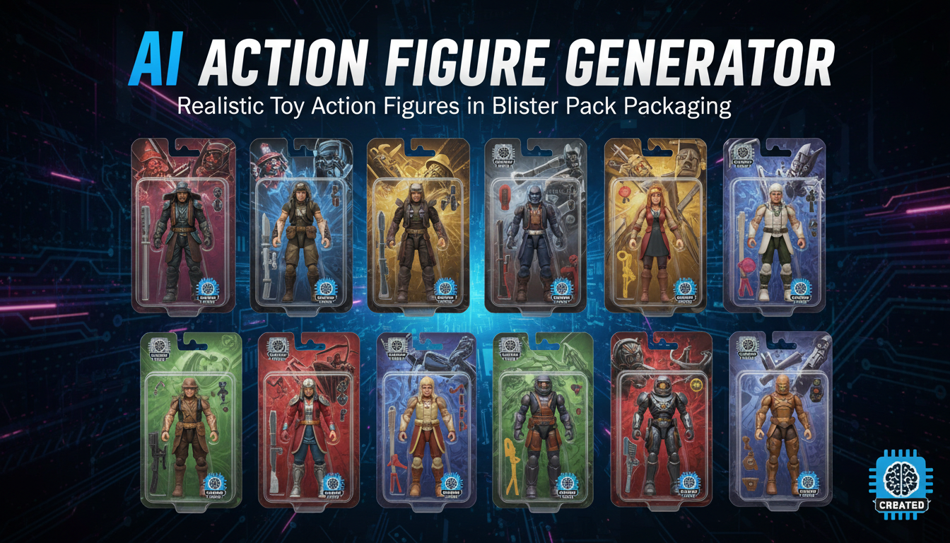
AI Action Figure Generator: How to Create Your Own Viral Toy Box Portrait in 2026
Complete guide to the AI action figure generator trend. Learn how to turn yourself into a collectible figure in blister pack packaging using ChatGPT, Flux, and more.